Data
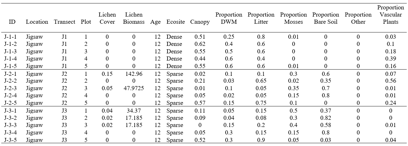
The raw data collected during the summer was entered into a master data table (Table 3). Each record in the table represents a 1 m² plot. The first four columns identify the plot using location, transect number and plot number. The two response variables are lichen cover (proportion) and total lichen biomass (g) for all species in the plot. Age and ecosite are predictor variables that were deliberately set as part of the sampling design. The remaining columns are covariates, since they were measured but not set as part of the sampling design. These covariates will be treated as predictor variables in later analyses to determine how they influence the response variables. Table 3 displays the data for the first 15 plots in the master data table. After data cleaning, the master data table contained 667 records.
Table 3. A sample of the master data table.
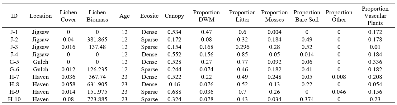
Following the convention of several previous studies (Arsenault et al. 1997; Dunford et al. 2006; McMullin et al. 2011), I created a summary table, where each record in the table represents a single transect (Table 4). The first two columns identify the transect by ID and location. Lichen cover (proportion) and lichen biomass (kg/ha) are the response variables. Lichen cover is the mean proportion lichen cover for the five plots on the transect. Lichen biomass in the sum of lichen biomass in all five plots on the transect, converted from g/5 m² to kg/ha. Age and ecosite are the two predictor variables. The remaining columns are covariates, that will be treated as predictor variables in later analyses. They were calculated as the mean value for the five plots on the transect. After data cleaning, the transect data table contained 134 records.
Table 4. A sample of the transect data table.
Exploratory Graphics
When selecting burns for sampling, I wanted representation across the continuum of time since fire, so I focused on ensuring representation from seven decadal classes (Figure 9). I sampled burns 20-50 years old in greater proportion to test the 40-year recovery threshold for woodland caribou habitat.
When selecting burns for sampling, I wanted representation across the continuum of time since fire, so I focused on ensuring representation from seven decadal classes (Figure 9). I sampled burns 20-50 years old in greater proportion to test the 40-year recovery threshold for woodland caribou habitat.
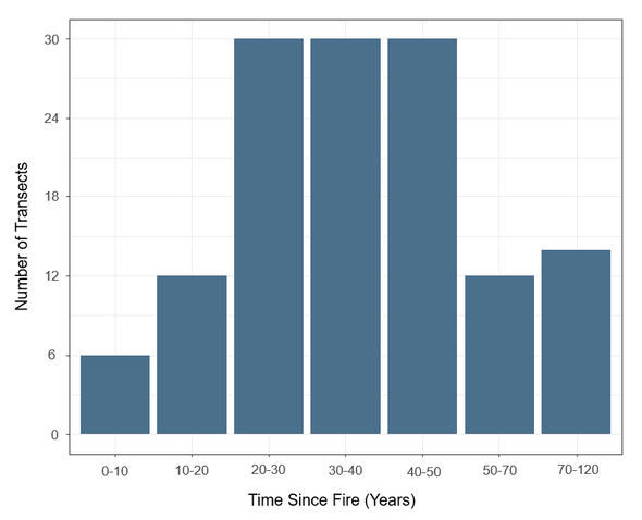
Figure 9. Number of transects for each time since fire class. 134 transects were sampled in total.
Since my study relies on cover-to-biomass conversion factors, I graphed lichen biomass as a function of lichen cover, and added a regression line to the plot to determine the direction and strength of the relationship between these two variables (Figure 10). The high R² value for the regression (R² = 0.98) indicates that lichen cover can explain almost all of the variation in lichen biomass. Labeling the points by ecosite revealed that plots in sparse conifer generally contained more lichen compared to plots in dense conifer.
Since my study relies on cover-to-biomass conversion factors, I graphed lichen biomass as a function of lichen cover, and added a regression line to the plot to determine the direction and strength of the relationship between these two variables (Figure 10). The high R² value for the regression (R² = 0.98) indicates that lichen cover can explain almost all of the variation in lichen biomass. Labeling the points by ecosite revealed that plots in sparse conifer generally contained more lichen compared to plots in dense conifer.
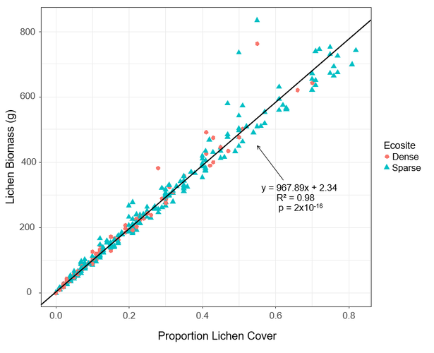
Figure 10. Cover-to-biomass relationship for all plots sampled.
I created two histograms to visualize the distribution of lichen biomass in the two different ecosites (Figure 11). Clearly, my data is not normally distributed. This is due to the prevalence of plots with little or no lichen, especially in dense conifer stands. I tried several transformations in an attempt to normalize the data, but the distribution never approached normality. Thus, I kept the values untransformed and use non-parametric statistics, including permutational ANOVA, to analyse the data.
I created two histograms to visualize the distribution of lichen biomass in the two different ecosites (Figure 11). Clearly, my data is not normally distributed. This is due to the prevalence of plots with little or no lichen, especially in dense conifer stands. I tried several transformations in an attempt to normalize the data, but the distribution never approached normality. Thus, I kept the values untransformed and use non-parametric statistics, including permutational ANOVA, to analyse the data.
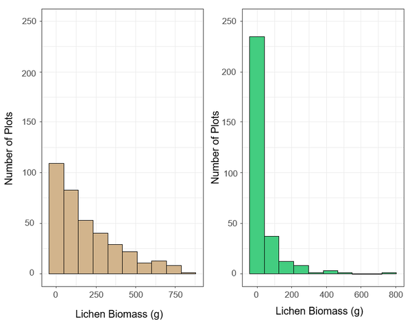
Figure 11. Histogram of plot-level lichen biomass (g) for sparse conifer (tan bars, n = 369) and dense conifer (green bars, n = 298).
