Methods
Field data for this study was collected in and around Woodland Caribou Provincial Park, in northwestern Ontario (Figure 3).
Field data for this study was collected in and around Woodland Caribou Provincial Park, in northwestern Ontario (Figure 3).
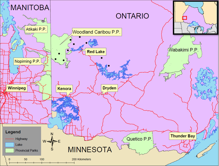
Figure 3. Regional context of the study area. Sample areas are indicated by black dots.
Sampling was stratified into burns of different ages, ranging from 2-119 years after fire (Figure 4). Within each burn, a minimum of three study sites were chosen in sparse conifer and three in dense conifer, resulting in a minimum of six study sites per burn.
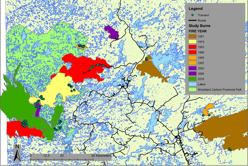
Figure 4. Study area for lichen sampling in and around Woodland Caribou Provincial Park. Each dot is a transect. Burns are coloured according to fire year. Age for sites originating before 1960 was acquired from a provincial Forest Resource Inventory.
At each study site, the starting point for a transect was established 25 m from the stand boundary. A transect tape was used to establish a transect 50 m in length. A 1 m² hoop plot was placed on the ground at each 10 m interval along the transect tape, for a total of 5 plots per transect (Figure 5).
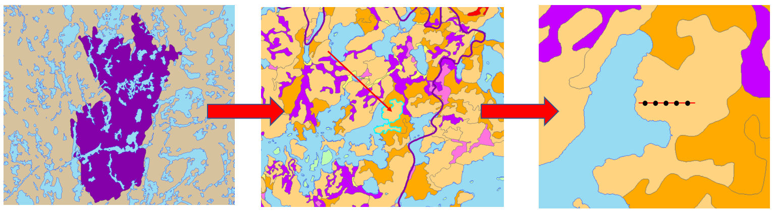
Figure 5. Site selection process. In this example, I chose to sample the purple burn (fire year = 2006, age = 12). Once I selected the burn, I used a forest inventory map to locate a sparse conifer polygon to sample (highlighted in blue with arrow). Then I established a 50 m transect (red line) and placed five 1 m² plots along it (black dots).
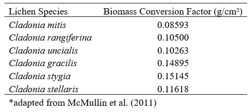
At each 1 m² plot, percent cover was estimated for the six species of ground lichens common in the region. Percent cover of vascular plants, downed woody material, litter, mosses, bare soil, rock and other materials was recorded for each plot. Canopy closure was estimated using a spherical densiometer. Percent cover of lichen was used to estimate lichen biomass at the plot and stand level using cover-to-biomass conversion factors developed by McMullin et al. (2011) (Table 1).
Table 1. Cover-to-biomass conversion factors used to estimate lichen biomass for the study area.
The conversion factors were verified for the study area by destructive lichen sampling. A 25 cm X 25 cm square subplot was placed within the 1 m² plot to cover a similar proportion of lichen as the 1 m² plot (Figures 6, 7). A total of 34 lichen samples were collected, sorted by species and dried and weighed in the lab. Conversion factors were determined by dividing the mass of the sample (g) by the cm² it covered, then taking the average g/cm² for each lichen species to derive the conversion factors.
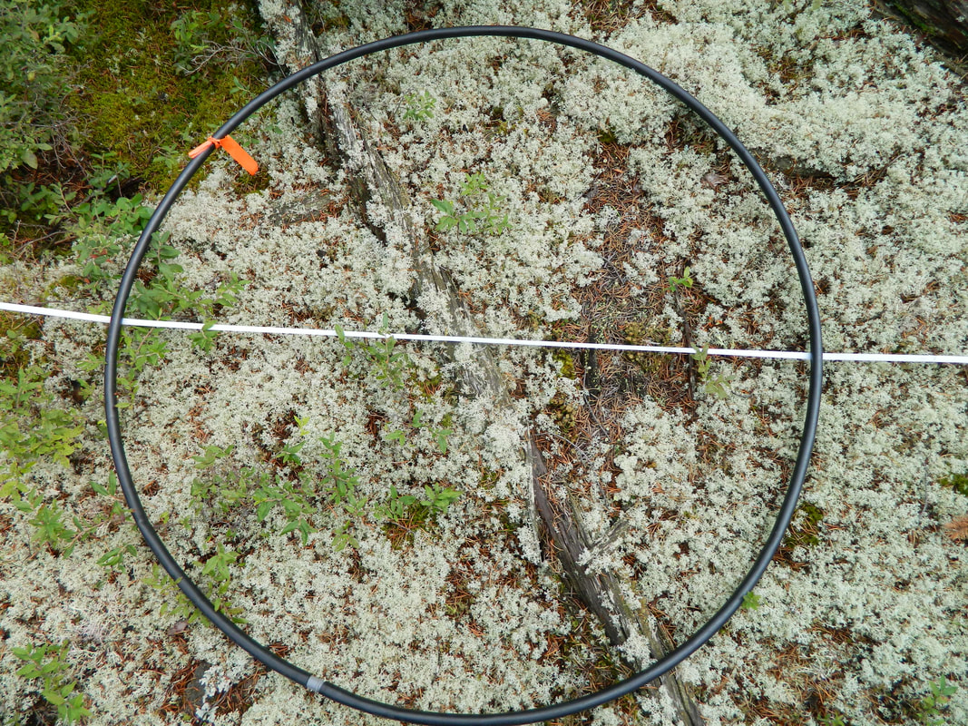
Figure 6. An example of a 1 m² hoop plot.
|
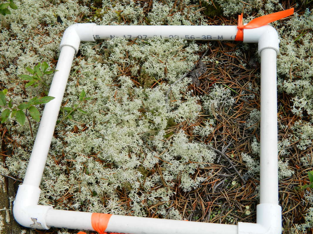
Figure 7. The corresponding subplot sample for the 1 m² plot in Figure 6.
|
Statistical Analysis
I used a series of two-tailed T-tests to validate the cover-to-biomass conversion factors created by McMullin et al. (2011). Using T-tests allowed me to detect whether the conversion factors I developed were significantly (α = 0.05) different than those developed by McMullin. Since I did not have McMullin’s raw data, I ran the T-tests manually using the methods taught in lecture instead of the t.test function in R.
I used a permutational ANOVA (lmPerm package, R version 3.4.3) to determine whether there are significant differences in lichen biomass with respect to age and ecosite. I decided to use a permutational ANOVA after inspecting the residual plot for lichen biomass and age (Figure 8). The residual plot demonstrates unequal variance, thus the non-parametric permutational ANOVA is a more appropriate choice as a statistical test.
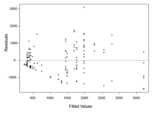
Figure 8. Residual plot of Lichen Biomass~Age. This plot demonstrates unequal variance.
I used piecewise regression (segmented package; R version 3.4.3) to determine the recovery threshold for lichen biomass in sparse conifer and dense conifer ecosites. Piecewise regression calculates a breakpoint, where the trend in the response variable changes abruptly. The function then calculates two linear relationships between the predictor variable and the response variable- one before the breakpoint and another after the breakpoint. This allows the user to visualize data with irregular or multiple trends, and the breakpoint can be used to empirically establish threshold values. In my analysis, I interpreted the breakpoint as the recovery threshold for lichen biomass following forest fires.
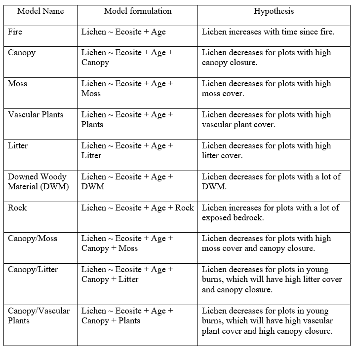
The next objective of my project is to map lichen abundance for my study area. To identify the variables that are most important in predicting lichen abundance, I created a set of ten hypotheses (Table 2). I tested these hypotheses by running a series of generalized linear mixed models on the plot-level data (glmmTMB package; R version 3.4.3). The response variable for the models was lichen abundance. Separate models were run with lichen biomass as the response variable (gamma distribution) and lichen cover as the response variable (beta distribution). The gamma distribution requires values > 0, so 0.01 was added to the lichen biomass values to ensure there were no zeros. The beta distribution requires values be between 0 and 1. The model cannot run with zeros or ones in the dataset, so the adjustment formula (Lichen Cover*(n-1) + 0.5)/n was applied to the data to satisfy this requirement (Cribari-Neto and Zeileis n.d.). All models included burn age and ecosite as fixed effects, since the levels of these variables were deliberately set as part of the sampling design. Transect ID was included as a random effect on all models to account for the dependence structure in the data (plots nested within transects).
Table 2. Model set used to identify the variables most important in predicting lichen abundance.
I used piecewise regression (segmented package; R version 3.4.3) to determine the recovery threshold for lichen biomass in sparse conifer and dense conifer ecosites. Piecewise regression calculates a breakpoint, where the trend in the response variable changes abruptly. The function then calculates two linear relationships between the predictor variable and the response variable- one before the breakpoint and another after the breakpoint. This allows the user to visualize data with irregular or multiple trends, and the breakpoint can be used to empirically establish threshold values. In my analysis, I interpreted the breakpoint as the recovery threshold for lichen biomass following forest fires.
The next objective of my project is to map lichen abundance for my study area. To identify the variables that are most important in predicting lichen abundance, I created a set of ten hypotheses (Table 2). I tested these hypotheses by running a series of generalized linear mixed models on the plot-level data (glmmTMB package; R version 3.4.3). The response variable for the models was lichen abundance. Separate models were run with lichen biomass as the response variable (gamma distribution) and lichen cover as the response variable (beta distribution). The gamma distribution requires values > 0, so 0.01 was added to the lichen biomass values to ensure there were no zeros. The beta distribution requires values be between 0 and 1. The model cannot run with zeros or ones in the dataset, so the adjustment formula (Lichen Cover*(n-1) + 0.5)/n was applied to the data to satisfy this requirement (Cribari-Neto and Zeileis n.d.). All models included burn age and ecosite as fixed effects, since the levels of these variables were deliberately set as part of the sampling design. Transect ID was included as a random effect on all models to account for the dependence structure in the data (plots nested within transects).
Table 2. Model set used to identify the variables most important in predicting lichen abundance.
Models were ranked using the Akaike Information Criterion (AIC) scores, with lower scores indicating a model with higher predictive capacity. Akaike weights and ∆AIC were also used to compare models. ∆AIC is the difference between the AIC score of model x and the AIC score of the top model. In general, models with a ∆AIC > 2 are considered significantly less informative than the model with the lower score (Harrsion et al. 2018). Akaike weights (wi) indicate the likelihood that each model is the best of the set. Akaike weights were calculated for each model according to the equation exp(-0.5*AICi)/sum(AIC) (O'Meara n.d.). The model summary was analysed in R to determine coefficient direction and standard errors. The two model sets were compared using the standard errors of the model coefficients and residual plots generated by the DHARMa package (R version 3.4.3).
